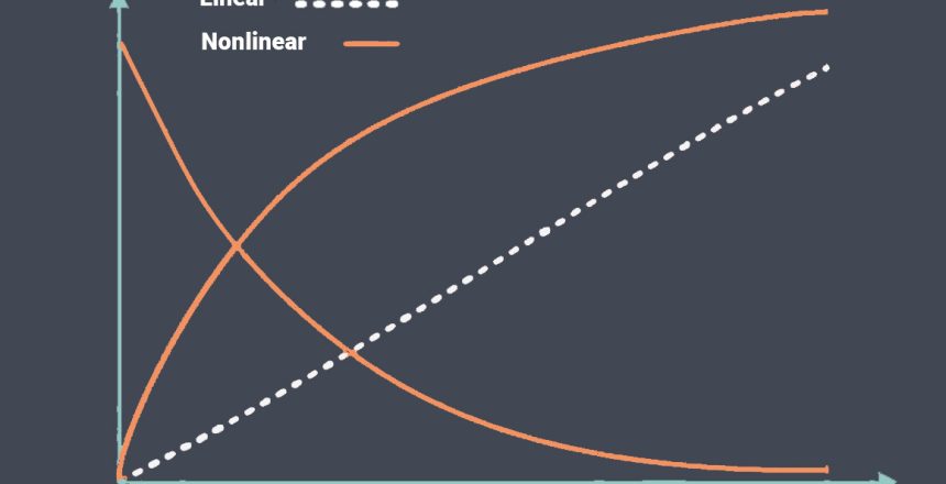
The sensor transfer function is a mathematical relationship that describes how the input signal to a sensor is transformed into the output signal. It is an equation or a graph that shows the relationship between the input and output signals of the sensor over a specified range of inputs.
The transfer function is a mathematical function which represents the relation between a physical measured parameter, also called stimulus or phenomenon. The system response which is an electrical output signal, whose relation can be expressed as S = f (p), where S is the electrical output signal and p is the stimulus.
Here are some examples of sensor transfer functions with their formulas:
Linear transfer function
In control systems engineering, a linear transfer function describes the relationship between the input and output signals of a system in a linear time-invariant (LTI) system. It is commonly used to represent the behavior of dynamic systems such as electrical circuits, mechanical systems, and chemical processes.
In a linear sensor, the output signal is directly proportional to the input signal.
The transfer function for a linear sensor can be expressed as:
S= as+b
where

S is the output signal,
s is the input signal,
a is the slope of the line
(sometimes called sensitivity)
b is the y-intercept
(i.e. output signal at zero input signal)
The transfer function describes how the system responds to different frequencies present in the input signal. It characterizes the system’s dynamics, including its gain (amplification or attenuation) and phase shift properties.
Linear transfer functions satisfy the properties of linearity, which means they follow the principles of superposition and homogeneity. Superposition states that the response to a sum of multiple inputs is equal to the sum of individual responses to each input separately. Homogeneity implies that scaling the input signal will result in a corresponding scaling of the output signal.
Nonlinear transfer function
A nonlinear transfer function is a mathematical relationship that describes the input-output behavior of a system or device where the output is not directly proportional to the input.
In other words, the output does not follow a linear relationship with the input.
In contrast to linear transfer functions, which can be represented by a straight line or a linear equation, nonlinear transfer functions exhibit

more complex and often nonlinear relationships between the input and output variables. These relationships can take various forms, such as exponential, logarithmic, polynomial, trigonometric, or piecewise-defined functions.
In general, these functions can be shown as follows:
Logarithmic transfer function

exponential transfer function

Power transfer function

Note: In all these equations, k is a constant number.
For example, the transfer function for a thermistor, which is a type of temperature sensor with a nonlinear resistance-temperature relationship, can be expressed as:
R = R0 * exp(B * (1/T – 1/T0))
Where
R is the resistance of the thermistor at temperature T,
R0 is the resistance of the thermistor at temperature T0,
B is a constant that depends on the material properties of the thermistor.
Note: Actually for nonlinear transfer functions, Unlike the linear relationship (The first equation), the slope of the line “m” (sensitivity factor) ; is not a constant number. For each X0 specific input value , it can be defined as follows:

Another important property of non-linear systems is that they can exhibit a wide range of phenomena that are not present in linear systems, such as chaos, bifurcations, and limit cycles. These phenomena can arise due to the non-linearities in the system, and can have important practical implications for system design and control.
Despite their complexity, non-linear systems are of great practical importance in many areas of engineering, science, and technology. For example, non-linear control systems are used in aerospace applications to control the position and orientation of spacecraft, and in robotics to control the motion and behavior of robots. Non-linear mechanical systems are used in the design of vehicles and structures to improve their performance and durability. Non-linear electrical systems are used in power electronics to control the flow of electrical power, and in renewable energy systems to convert and store energy from renewable sources.
Piecewise transfer function
In some sensors, the transfer function may be piecewise, meaning that it has different functional forms in different regions of the input range. In other words, the function “switches” from one expression to another at certain points in the input domain, resulting in a piecewise-defined function. A piecewise transfer function can be expressed as a set of equations, with different equations for different regions of the input range.
Piecewise transfer functions are commonly used in control systems and signal processing applications, where different mathematical models may be appropriate for different parts of the input domain.
For example, the transfer function for a load cell, which is a type of force sensor, may have different equations for different regions of the load range. In the lower load range, the transfer function may be linear,

while in the higher load range, the transfer function may be nonlinear. The piecewise transfer function can be expressed as a set of equations for each region of the input range.
A simple example of a piecewise transfer function is the absolute value function, which is defined as:
f(x) = |x| if x < 0
f(x) = x if x >= 0
This function has a different mathematical expression for x < 0 and x >= 0, resulting in a piecewise-defined function. Another example is the “signum” function, which returns the sign of the input:
f(x) = -1 if x < 0
f(x) = 0 if x = 0
f(x) = 1 if x > 0
Piecewise transfer functions can be analyzed and manipulated using techniques similar to those used for other types of mathematical functions, such as integration, differentiation, and Fourier analysis. However, special care must be taken to ensure that the function is continuous and differentiable at the points of transition between the different mathematical expressions.

